Schema selection
Overview
It is common for enterprise databases to use multiple schemata to partition the data, it is either separated by business domain or some other context.
This is especially true for Data warehouses. It is rare when the default schema is going to have all of the data needed for an analysis.
For analyses using dplyr, the in_schema() function should cover most of the cases when the non-default schema needs to be accessed.
An example
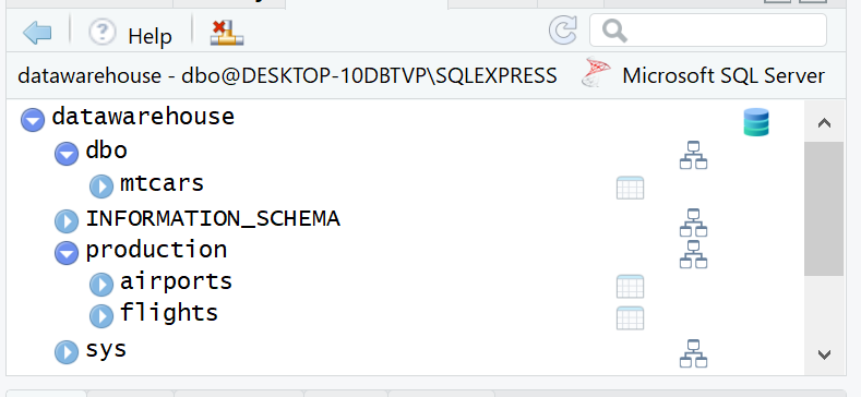
The following ODBC connection opens a session with the datawarehouse database:
con <- DBI::dbConnect(odbc::odbc(), "datawarehouse")The database contains several schemata. The default schema is dbo. So to it is very straightforward to access it via dplyr. The difficulty occurs when attempting to access a table not in that schema, such as tables in the production schema.

This is how to access a table inside the dbo schema, using dplyr:
library(dplyr)
library(dbplyr)

tbl(con, "mtcars") %>%
  head()
## # Source: lazy query [?? x 12]
## # Database: Microsoft SQL Server
## # 14.00.1000[dbo@DESKTOP-10DBTVP\SQLEXPRESS/datawarehouse]
## row_names mpg cyl disp hp drat wt qsec vs am gear
## <chr> <dbl> <dbl> <dbl> <dbl> <dbl> <dbl> <dbl> <dbl> <dbl> <dbl>
## 1 Mazda RX4 21.0 6. 160. 110. 3.90 2.62 16.5 0. 1. 4.
## 2 Mazda RX4 W~ 21.0 6. 160. 110. 3.90 2.88 17.0 0. 1. 4.
## 3 Datsun 710 22.8 4. 108. 93. 3.85 2.32 18.6 1. 1. 4.
## 4 Hornet 4 Dr~ 21.4 6. 258. 110. 3.08 3.22 19.4 1. 0. 3.
## 5 Hornet Spor~ 18.7 8. 360. 175. 3.15 3.44 17.0 0. 0. 3.
## 6 Valiant 18.1 6. 225. 105. 2.76 3.46 20.2 1. 0. 3.
## # ... with 1 more variable: carb <dbl>The same approach does not work for accessing the flights table, which resides in the production schema:
tbl(con, "flights")Error: <SQL> 'SELECT * FROM "flights" AS "zzz2" WHERE (0 = 1)' nanodbc/nanodbc.cpp:
1587: 42S02: [Microsoft][ODBC SQL Server Driver][SQL Server]Invalid object name
'flights'.Using in_schema()
The in_schema() function works by passing it inside the tbl() function. The schema and table are passed as quoted names:
tbl(con, in_schema("production", "flights")) %>%
  head()
## # Source: lazy query [?? x 29]
## # Database: Microsoft SQL Server
## # 14.00.1000[dbo@DESKTOP-10DBTVP\SQLEXPRESS/datawarehouse]
## year month dayofmonth dayofweek deptime crsdeptime arrtime crsarrtime
## <int> <int> <int> <int> <int> <int> <int> <int>
## 1 2006 1 11 3 743 745 1024 1018
## 2 2006 1 11 3 1053 1053 1313 1318
## 3 2006 1 11 3 1915 1915 2110 2133
## 4 2006 1 11 3 1753 1755 1925 1933
## 5 2006 1 11 3 824 832 1015 1015
## 6 2006 1 11 3 627 630 834 832
## # ... with 21 more variables: uniquecarrier <chr>, flightnum <int>,
## # tailnum <chr>, actualelapsedtime <int>, crselapsedtime <int>,
## # airtime <int>, arrdelay <int>, depdelay <int>, origin <chr>,
## # dest <chr>, distance <int>, taxiin <int>, taxiout <int>,
## # cancelled <int>, cancellationcode <chr>, diverted <int>,
## # carrierdelay <int>, weatherdelay <int>, nasdelay <int>,
## # securitydelay <int>, lateaircraftdelay <int>Ideal use
For interactive use, we would avoid using the tbl() command at the top of every dplyr piped code set. So it is better to load the table pointer into a variable:
db_flights <- tbl(con, in_schema("production", "flights"))An additional advantage of loading a variable with the table reference is that the field auto-completion is activated. This happens because the vars attribute, from the tbl() output, is loaded in the variable.
The operations that follow become more natural for a dplyr user
db_flights %>%
  group_by(month) %>%
  summarise(
    canceled= sum(cancelled, na.rm = TRUE),
    total = n()) %>%
  arrange(month)
## # Source: lazy query [?? x 3]
## # Database: Microsoft SQL Server
## # 14.00.1000[dbo@DESKTOP-10DBTVP\SQLEXPRESS/datawarehouse]
## # Ordered by: month
## month canceled total
## <int> <int> <int>
## 1 1 25564 1202846
## 2 2 36758 1096851
## 3 3 24463 1244426
## 4 4 17742 1199999
## 5 5 13898 1234528
## 6 6 27331 1227595
## 7 7 24241 1269804
## 8 8 22078 1282011
## 9 9 16457 1185124
## 10 10 18726 1241710
## # ... with more rowsWriting data
The copy_to() command defaults to creating and populating temporary tables. So when used with in_schema(), the most likely result is that the command will be ignored, and a table called “[schema].[table]” is created.
copy_to(con, iris, in_schema("production", "iris"))Created a temporary table named: ##production.irisEach enterprise grade database has its own way to manage of temporary tables. So the best course of action is to relay on the those mechanisms, and just request a temporary table.
db_iris <- copy_to(con, iris)

head(db_iris)
## # Source: lazy query [?? x 5]
## # Database: Microsoft SQL Server
## # 14.00.1000[dbo@DESKTOP-10DBTVP\SQLEXPRESS/datawarehouse]
## Sepal.Length Sepal.Width Petal.Length Petal.Width Species
## <dbl> <dbl> <dbl> <dbl> <chr>
## 1 5.10 3.50 1.40 0.200 setosa
## 2 4.90 3.00 1.40 0.200 setosa
## 3 4.70 3.20 1.30 0.200 setosa
## 4 4.60 3.10 1.50 0.200 setosa
## 5 5.00 3.60 1.40 0.200 setosa
## 6 5.40 3.90 1.70 0.400 setosaIn this particular case, the iris dataset was copied to the tempdb database, but in a mirror schema called production
Write non-temporary tables
The best way to create a permanent table, inside a specific schema, is to use the DBI package. The dbWriteTable() and SQL() commands should accomplish the task:
library(DBI)

dbWriteTable(con, SQL("production.iris"), iris)
DBI::dbDisconnect(con)